Teachers:
In this computer lab you will analyze a public AIRRseq (Adaptive Immune Receptor Repertoire Sequencing) dataset using the Immcantation software suite. The computer exercises are performed on the SurfSara Research Cloud. A system such as cloud or a computer cluster is what you would normally need to analyze AIRRseq datasets.
First you need to login to the SurfSara Research Cloud. Most bioinformatics software is developed for Linux systems. The "virtual machine" that you will work on has all software pre-installed that you need for the exercises (consult the Immcantation documentation if you would like to install/use the software yourself).
You have received a SSH key by e-mail. You need this file to login to cloud.
By mail you have also received a username (studentXX, where XX is a number) and an ip-address (which looks like 145.38.205.87).
In the tutorial below change studentXX with the username that was assigned to you and the ip-address that was in the mail.
Store the SSH key that you have received by mail in directory ~/.ssh/ on your own laptop. Start the program called "Terminal". You will see a black window appear (it can have another colour), where you can type commands.
Make the SSH key file only readable for yourself like this:
chmod 600 ~/.ssh/id_rsa_cloud_student
With the following command you can login to cloud (change studentXX and ip-address with the login details that was send to you by mail):
ssh -i ~/.ssh/id_rsa_cloud_student studentXX@145.38.205.87
If the login succeeded your prompt (the line after which you can type commands) should look similar to this:
student01@arcaid:~$
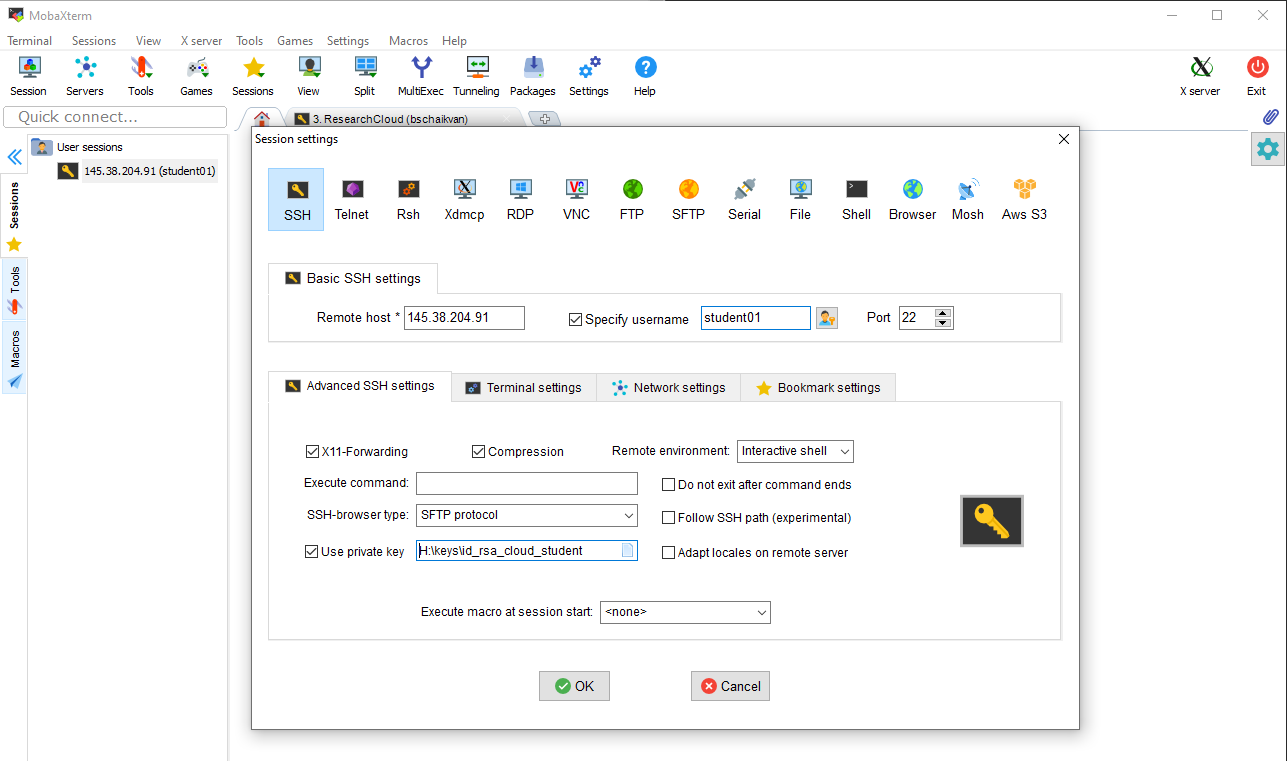
Windows does not have a program called "Terminal", so you will need to install a program to make the connection to cloud. Download and install the portable version of MobaXterm: https://mobaxterm.mobatek.net/download-home-edition.html
Store the SSH key that your have received by mail on your computer. Create a new session in MobaXterm and specify the location of the SSH (private) key as shown in the screenshot. Use the login name (studentXX) and ip-adress/host that was send to you by mail.
Some of you might not have worked on a Linux system before. These commands will help you to navigate through the system. Please note that every command you type is case sensitive!
The content of the current directory can be shown with the command ls. Using only ls will show you a condensed directory listing, the -l option (there is a space between ls and the option -l) shows you more details, such as the owner of the directory (student05 in this case) and date of creation (Feb 28 in this example).
ls -l
In this case there are only two directories (data and scratch), because we didn't do anything yet. It looks like this:
student05@arcaid:~$ ls -l
total 0
lrwxrwxrwx 1 student05 student05 5 Feb 28 09:32 data -> /data
lrwxrwxrwx 1 student05 student05 8 Feb 28 09:32 scratch -> /scratch
To go to another directory you can use the cd (Change Directory) command.
cd data
After hitting enter you will see that the prompt has changed. The name of the directory (data) is now part of the prompt.
student05@arcaid:~$ cd data
student05@arcaid:~/data$
Again you can see the content with ls -l. You will see the subdirectory "datasets". Go to this directory with the cd command. You will notice that the prompt changed again. By looking at the prompt you know exactly where you are on the system.
student05@arcaid:~/data$ cd datasets
student05@arcaid:~/data/datasets$
To move one directory up you need the command cd .. (notice the double dots, this means that you will navigate to the parent directory). To go back to your "home" directory simply type cd without specifying a directory.
student05@arcaid:~/data/datasets$ cd ..
student05@arcaid:~/data$ cd
student05@arcaid:~$
There are many good introduction tutorials on linux on the internet. We will keep the virtual machine running this week, so feel free to extend your linux skills using this cloud machine.
Typically, the steps that you will take for analyzing an AIRRseq dataset are the following.
We will use the first 25000 sequences of one sample of a publicly available dataset.
Before you start, make sure that you are in your home directory:
cd
Fastq-dump is part of the SRA toolkit. You can use this to fetch public datasets from NCBI's SRA. We will retrieve one sample. The -X indicates that we will only download the first 25000 sequences. The sequences will be split into the two read pairs with the option --split-files. The option --outdir specifies in which directory the files should be stored. SRR13107525 is the accession code (unique identifier) for the dataset that we are downloading.
fastq-dump --split-files -X 25000 --outdir sequences SRR13107525
A general remark: some steps take time (up to 10 or 15 minutes during this tutorial). Every time you will need to wait till the process is finished. You can see that you need to wait, because you prompt is not visible yet. Once it is visible you can continue with the next step.
When the download is complete (and your prompt is back) check which files were downloaded with:
ls -l sequences
The developers of the Immcantation software (the Kleinstein group) have provided their software in a so-called Docker container. It is a virtual environment where all the software and dependencies are pre-installed.
Here is a brief explanation about Docker (you can skip this, but it might be interesting for you as soon as are developing your own software): https://www.docker.com/
A description of the Docker container that is provided by the Kleinstein group can be found here: https://immcantation.readthedocs.io/en/stable/docker/intro.html PS, you don't have to follow the steps on this page because it is already on the cloud machine.
An overview of the Immcantation suite is here: https://immcantation.readthedocs.io/ Please have a look at this page to see what you can do with the Immcantation software.
With the sudo docker command we can start the docker container. The directory with the data ("sequences") is connected to the docker container with the -v option. Once inside the docker container the data will be available in the directory "data".
sudo docker run -it -v $HOME/sequences:/data:z immcantation/suite:4.3.0 bash
cd /data
Your prompt should look similar to this:
[root@a7e956d208f9 data]#
And if you type ls -l you should see the two fastq files.
The data that you have downloaded is a paired-end RNAseq experiment where the B cell receptors from peripheral blood were sequenced from an individual with moderate Covid-19 symptoms. The two ends of the pair overlap each other and the first step in the analysis is to assemble these ends into complete sequences. This can be done with pRESTO. Please have a look at this website for a description of the pRESTO pipeline.
https://presto.readthedocs.io/en/stable/workflows/Greiff2014_Workflow.html
With AssemblePairs.py you will perform a pairwise assembly of the sequences that you have downloaded before. The second command creates a quality report of the assembly. Once the analysis is complete (when you have your prompt back) check which files were created with the ls command.
AssemblePairs.py align -1 SRR13107525_1.fastq -2 SRR13107525_2.fastq --coord sra --rc tail --outname test --log AP.log
ParseLog.py -l AP.log -f ID LENGTH OVERLAP ERROR PVALUE
ls -l
You can see the content of files with the less command. By hitting the space bar you scroll through the file. To exit you press q. Have a look at the produced assembly report with:
less AP_table.tab
pRESTO has scripts to filter out low quality sequences. This is done with the program FilterSeq.py
FilterSeq.py quality -s test_assemble-pass.fastq -q 20 --outname test --log FS.log
ParseLog.py -l FS.log -f ID QUALITY
Again, inspect which files were created with ls and look at the content of the created files using less.
The primer sequences are unknown for this dataset, so this step is ommited during this tutorial. In case you would like to analyze somatic hypermutation it can be wise to mask the primer sequences, because you could get biased results if you don't. If you do know the primers you could mask them as follows, where the primer sequences are specified in the files "VPrimers.fasta" and "CPrimers.fasta".
MaskPrimers.py score -s test_quality-pass.fastq -p VPrimers.fasta --start 4 --mode mask --pf VPRIMER --outname test-FWD --log MPV.log
MaskPrimers.py score -s test-FWD_primers-pass.fastq -p CPrimers.fasta --start 4 --mode cut --revpr --pf CPRIMER --outname test-REV --log MPC.log
ParseLog.py -l MPV.log MPC.log -f ID PRIMER ERROR
IgBLAST uses sequences in FASTA format and the experiment sequences are currently in FASTQ format, so you will need to convert the sequences from FASTQ to FASTA format first.
You can read more about FASTA and FASTQ here.
Read more about the IgBLAST step here: https://changeo.readthedocs.io/en/stable/examples/igblast.html
fastq2fasta.py test_quality-pass.fastq
Once you have your sequences in FASTA format you can execute IgBLAST.
AssignGenes.py igblast -s test_quality-pass.fasta -b /usr/local/share/igblast --organism human --loci ig --format blast
For the next step (clustering sequences with Change-O) the IgBLAST output needs to be reformatted:
MakeDb.py igblast -i test_quality-pass_igblast.fmt7 -s test_quality-pass.fasta -r /usr/local/share/germlines/imgt/human/vdj/imgt_human_IGHV.fasta /usr/local/share/germlines/imgt/human/vdj/imgt_human_IGHD.fasta /usr/local/share/germlines/imgt/human/vdj/imgt_human_IGHJ.fasta --extended
Non-productive sequences can be removed like this:
ParseDb.py select -d test_quality-pass_igblast_db-pass.tsv -f productive -u T
To get an idea about clonal expansion or if you would like to create lineage trees of related B cells you would like to know which B cell receptors belong to the same clone group (clonal family). This is usually done by grouping B cell receptors that have a high similarity. With the assumption that similar sequences belong to the same B cell clone. There are several methods available to do this. Dasha can tell you all about it. In this tutorial we will use Shazam and Change-O.
Short description of these methods:
https://changeo.readthedocs.io/en/stable/examples/cloning.html
https://shazam.readthedocs.io/en/stable/vignettes/DistToNearest-Vignette/
In the first step we need to determine a threshold for grouping sequences together. With the Shazam R package distances between all sequences can be determined and a threshold for sequences that have a high similarity.
Start R
R
Your prompt should look like this now:
R version 4.0.5 (2021-03-31) -- "Shake and Throw"
Copyright (C) 2021 The R Foundation for Statistical Computing
Platform: x86_64-redhat-linux-gnu (64-bit)

R is free software and comes with ABSOLUTELY NO WARRANTY.
You are welcome to redistribute it under certain conditions.
Type 'license()' or 'licence()' for distribution details.

R is a collaborative project with many contributors.
Type 'contributors()' for more information and
'citation()' on how to cite R or R packages in publications.

Type 'demo()' for some demos, 'help()' for on-line help, or
'help.start()' for an HTML browser interface to help.
Type 'q()' to quit R.

>
Load the shazam library and the data.
library(shazam)
df<-read.csv(file='test_quality-pass_igblast_db-pass_parse-select.tsv', sep='\t')
Calculate the Hamming distance between the sequences and determine the threshold of unrelated vs related sequences.
dist_ham<-distToNearest(df, sequenceColumn="junction", vCallColumn="v_call", jCallColumn="j_call", model="ham", normalize="len", nproc=1)
output <- findThreshold(dist_ham$dist_nearest, method="density")
threshold<-output@threshold
threshold
q()
Write down the threshold for later use in DefineClones.py.
When you quit R, the program asks you whether you want to save the workspace: n for no.
With the DefineClones.py program you can group sequences that are similar into clonal families. In the example below the threshold 0.1105961 is used. You should use the threshold that came out of shazam.
DefineClones.py -d test_quality-pass_igblast_db-pass_parse-select.tsv --act set --model ham --norm len --dist 0.1105961
Quit Docker by typing exit. Now your prompt should look like this:
student01@arcaid:~$
The results of the analysis you just did can be found in the directory "sequences". Check this by using the ls command.
ls -l sequences/
Download the test_quality-pass_igblast_db-pass_parse-select_clone-pass.tsv file as follows.
Windows
If you are using MobaXterm you can do this via the file panel on the left (you might need to refresh the file explorer first). Just drag&drop the file to your desktop.
Linux or Mac
You can download the file using the scp command. First exit the virtual machine by typing exit.
Download the file with scp. Don't forget the space and the dot at the end of this command.
scp -i ~/.ssh/id_rsa_cloud_student studentXX@145.38.205.87:~/sequences/test_quality-pass_igblast_db-pass_parse-select_clone-pass.tsv .
Plan B
If you are not able to download the file, then you can download it HERE.
Now open the file in Excel, LibreOffice or some other spreadsheet program (Google spreadsheet might work for you if you do not have a spreadsheet program on your laptop. In this example Google Spreadsheet is used, but other spreadsheet programs have the same functionality.
Count the number of sequences per clonal family by creating a "pivot table".
=if(C2>0.5, 1, 0))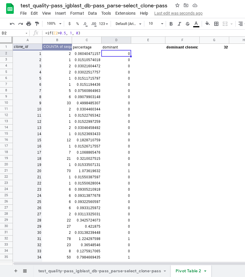
If you have made it this far: congratulations!
During these exercises you have worked with a smaller dataset. Usually the dataset is approximately ten times (or more) larger and typically you will analyze multiple datasets. You went through all the data analysis steps one by one by typing commands. This is something you would normally put in a python or bash script with loops, etc, to process all datasets at once.
These data analysis steps are the starting point for further analysis. E.g. creating lineage trees, comparing clonal families between samples, analyzing somatic hypermutations, and much more. The development of methods for AIRRseq data goes fast and there is a need for standardization. If you want to be kept informed about the advances in the field, keep an eye on news from the AIRR community.